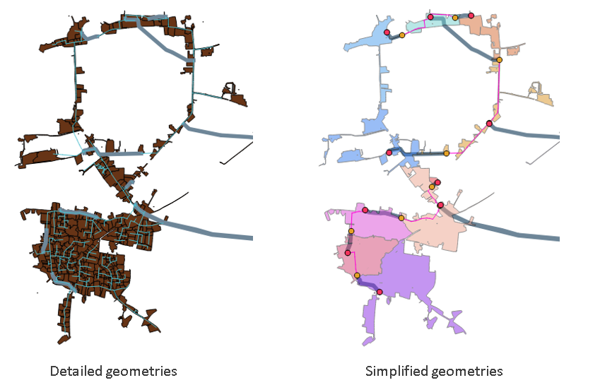
Support for rich and extensible data types

Introduction

This is part of a series of articles where we describe the way the Meniscus Analytics Platform (MAP) works. Theses articles jump into the features that make MAP different to other analytics applications by providing an Integrated Analytics Stack delivering real time analytics. IN this article we talk about extensible data types.

This article discusses how and why having extensible data types is a real benefit when developing your analytics applications

Why are extensible data types important?

Being able to use a wide variety of ‘standard’ data types, but also to create your own, delivers lots of benefits.

  • Provides flexibility. During the import stage you can re-process and store the initial raw data into a ‘pre-processed’ data type. When you want to use this data to deliver a calculation or other use then the data is already configured and available in exactly the format you want
  • Greatly increases data processing and calculation times.
  • Extensible data types give you the ability to control how you store and process your raw data

Examples of data types supported by MAP

We have a number of ‘standard’ extensible data types already configured in MAP but there is no limit to the number or variety that you can create.

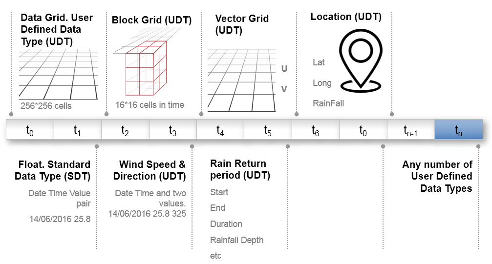
  • Data Grid. One of the most important for our MAP Rain solution. Processes data in any size of two dimensional grid. Used for radar and forecast rainfall data, satellite imagery and the like
  • Block Grid. Used in conjunction with a Data Grid. Breaks a two dimensional Data Grid into a smaller three dimensional Block. Used for speeding up the processing of Data Grids by ensuring MAP only processes relevant data. See article on lazy loading of data sets
  • Vector Grid. Similar to a Data Grid but provides a two dimensional grid but includes vector and direction data as well. Used for processing grids of forecast wind speed and direction data.
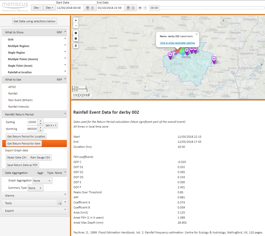
  • Rainfall Location. Holds the location of a point of interest (Latitude and Longitude) as well as the current and historic rainfall data for that Location. Used in MAP Rain
  • Float – standard time series. This is a standard data type for processing time series data. Contains a Date/Time Value pair
  • Journey. Used to create and store a sequence of locations along the route of a journey. We use this data type to predict rainfall along this route using our Hyperlocal rainfall product

Examples of data types

About MAP

MAP is an Integrated Analytics Stack providing a framework for users to create and deploy calculations at scale using any source of raw data. MAP is based on IOT principles and uses Items as the underlying building blocks to store either RAW or CALCulated data. So, users create an Entity Template or Thing using these Items and then replicate this template hundreds of thousands of times using an ItemFactory.

For more information on MAP then click here

Benefits of a dynamically constructed dependency tree

Introduction

This is part of a series of articles where we describe the way the Meniscus Analytics Platform (MAP) works. Theses articles jump into the features that make MAP different to other analytics applications by providing an Integrated Analytics Stack delivering real time analytics. This article discusses the benefits of a dynamically constructed dependency tree.

What is a dynamic dependency tree?

A dependency tree is a list or tree of the way that any Item links to other Items. We use this to manage and understand which Items are required when calculating another Item. So, if Item 1 requires Item 3 and Item 2004 to calculate then any change in Item 3 or Item 2004 will place Item 1 on the calculation queue to be recalculated. The process of managing the Items placed on the queue is critical to MAP and we have a separate Invalidator module specifically to do this.

While our old MCE analytics platform held a dependency tree it was not dynamic and so, not really a scalable solution. MAP uses a dynamic dependency tree so that as new Items are added then MAP automatically creates its own tree by learning from the calculations as they run. This in turn means that MAP is scalable and can run on any size of database.

Benefits of using a dependency tree

  • Calculation speed. By knowing the relation between each and every Item ensures MAP processes data in the most optimal way possible. This is turn helps to ensure MAP can deliver lightning fast calculation speeds
  • Automated. Being an automated process means that a developer can just leave MAP to get on and do it’s own ‘thing’ whilst they focus on the critical aspects of developing their application

About MAP

MAP is an Integrated Analytics Stack providing a framework for users to create and deploy calculations at scale using any source of raw data. MAP is based on IOT principles and uses Items as the underlying building blocks to store either RAW or CALCulated data. So, users create an Entity Template or Thing using these Items and then replicate this template hundreds of thousands of times using an ItemFactory.

For more information on MAP then click here

Using Data Blocks and Data Versioning to deliver real time analytics

Introduction

This is part of a series of articles where we describe the way the Meniscus Analytics Platform (MAP) works. Theses articles jump into the features that make MAP different to other analytics applications by providing an Integrated Analytics Stack delivering real time analytics. In this article we discuss Data Blocks and Data Versioning.

In delivering real time analytics, disk IOPS (Input/output Operations Per Second) is one of the main rate limiting steps in achieving the calculation speeds required when processing high volume and high velocity raw data. An example of such a data is radar rainfall data where new values covering a large area arrive every 5 minutes.

To help reduce disk IOPS, we developed the concepts of Data Blocks and Data Versioning into MAP to drastically speed up data access, increase calculation speed and reduce the volume of data written back to the database.

Data Blocks

Rather than loading and persisting all data for an Item, data can be broken up into chunks called Blocks. So, only the chunks of data that are demanded for a query, or as an input to a calculation, are loaded from the database (i.e. delay loading), and only the chunks of data that actually change need to be persisted. Blocks are typically used with unbounded, time-related data such as sample arrays, where the size of a Block is limited and the maximum number of Block samples depends on the size of a sample. This provides efficiencies in real-time processing, whereby data changes are localised and typically at the end of the data.

Data Blocks are transparent to the user. It is purely an internal mechanism to reduce traffic to/from the database. When requested or persisted, Data Blocks are held in memory for a time. This ensures future retrieval is temporarily faster as the data is expected to be in demand.

Data Versioning

Data Blocks are complimented by the MAP concept of Data Versioning. All Item data in MAP is versioned, including Blocks (as such referred to as child data). A version is simply a unique timestamp. It allows users to query for the relative age of data. Specifically, when it last changed, and for calculated Items when the last calculation started and completed. A client application can then tell if data has changed without having to load the data itself. There are additional non-data versions on an Item. I.E when its properties or list of child items last changed.

It is this versioning technique that allows MAP to efficiently detect when calculated items need recalculating (referred to as dirtying as calculation).

About MAP

MAP is an Integrated Analytics Stack providing a framework for users to create and deploy calculations at scale using any source of raw data. MAP is based on IOT principles and uses Items as the underlying building blocks to store either RAW or CALCulated data. So, users create an Entity Template or Thing using these Items and then replicate this template hundreds of thousands of times using an ItemFactory.

For more information on MAP then click here

MAP Sewer – creation of simplified sewer network models

New MAP Sewer capability speeds up the creation of the simplified sewer network models. This makes is quicker and easier to set up our near real time predictive modelling of the sewer network.

We have been working to speed up the creation of the simplified sewer network models in MAP Sewer so that we can rapidly create new models for new catchments. We have now automated the process of creating the main simplified model, and all the relevant geometries, from the detailed GIS layers that make up the ‘standard’ detailed models used by most water companies.

The objective of this work is:

  • Generate the MAP Sewer model inputs from the detailed model
  • To do this in an automated way using a combination of QGIS and PYTHON scripts
  • The methodology includes:

  • Derive location of Pumping Stations, Combined Sewer Overflows, Detention tanks, Weirs and Sluices
  • For each Pumping Station, use QGIS flow trace to identify the upstream conduits
  • Identify the sub-catchments associated to these upstream conduits
  • Dissolve the sub-catchments into one large sub-catchment
  • Aggregate the key sub-catchments properties
  • Calculate the main trunk sewer path and aggregate sewer length, gradient and diameter
  • Create the MAP Sewer nodes
  • The process takes several hours to run and the outputs are:

  • MAP Sewer configuration files. These are CSV files for each geometry. I.e. Pumping Stations, Combined Sewer Overflows, Detention tanks, Weirs and Sluices
  • One sub-catchment file containing all the dissolved sub-catchments. this is a KML file
  • Once this is done then we can add some of the pumping attributes to the Pumping Station and Detention Tank geometry files and then load all the files into MAP Sewer from the dashboard. MAP Sewer then creates the geometries in a few minutes and the whole catchment is calculated in 20 minutes – this includes over 2 years of historic data all at 5 minute periodicity. We can now start to validate the model and to feed it with real time and forecast rainfall data.

    Optimize battery storage by predicting power output

    Case study – Short term solar irradiance predictions and impact on PV site revenue

    This case study summarises the work completed in an InnovateUK collaborative research project to optimize battery storage at PV sites using short term solar irradiance predictions. As a result of this work, the project delivered the following outcomes.

  • Deliver solar irradiance predictions for the next 2 1/2 hours at 15 minute intervals using the latest satellite imagery
  • Understand the relationship between solar irradiance and inverter output power
  • Model how short term solar power and solar irradiance predictions can increase revenue from Demand Side Response (DSR) schemes
  • Use this data to optimize battery storage
  • Quantify the financial benefits and the break even point in terms of site of PV site
  • The project uses near real time satellite imagery to predict the path of clouds and to predict the solar irradiance at any location for the next 2 hours at 15 minute increments. Therefore, by predicting the solar irradiance we can predict the solar power output for the site and optimize battery storage and increase revenue from the National Grid’s Demand Side Response programme.

    The Project found that PV sites larger than 2MW would benefit from this technology and it is especially coct effective for sites operating ‘behind the meter’ with either battery storage or with on-site demand.

    The project finished in January 2019 and was built using the Meniscus Analytics Platform (MAP).

    Project partners:

  • Meniscus Systems Ltd: Lead Partner providing the data analytics and processing capability to deliver solar irradiance predictions
  • Open Energi: Providing expertise to deliver accurate, real-time PV-based DSR solutions to DNOs and owner/operators of solar farms
  • BRE National Solar Centre: Responsible for ensuring the system meets the requirements of the PV industry. Providing domain expertise and access/advice on technical solar issues.
  • Cornwall Council: Owner/operator of one of the solar farms used to test and demonstrate the system
  • MAP Rain – New FEH 2013 Rainfall Return Period calculator

    FEH is the industry standard used to estimate local flood risk and develop resilient infrastructure.

    New Service – Rainfall Return Period calculation for any location using the FEH 2013 methodology

    MAP Rain dashboard and rainfall map now includes the updated FEH (Flood Estimation Handbook) 2013 methodology as well as the original FEH99 method. This provides the Return Period calculation for any location and any date in the past 4 years using the MAP Rain dashboard. These Return Period calculations are available for both Points and Polygons.

    You can use the MAP Rain dashboard to calculate:

  • The depth (mm) and duration (hours) of rainfall that generates the largest Return Period on a particular day
  • The depth (mm) of rain for the location that generates a specific Return Period for a specific rainfall duration (hours)
  • For more information on our MAP Rain dashboard and rainfall map click here

    Predicted Rainfall Alerts
    MAP Rain can also apply the FEH 2013 methodology to the forecast rainfall so that we can send you e-mail alerts for any significant rain events that may impact flooding hotspots.

    Return Period calculation API calls

    We have built two API calls into MAP to let you integrate the FEH 2013 return period calculations directly into your own applications. Please note that these call will take about 2 minutes to return.

    Returns depth (mm), duration (hours) and Return Period for a particular day and location

    Inputs

    Date 17th Sept 2017 (rainy day)
    Location in Long Lat (WGS84) or OS Easting and Northing

    Returns

    Rain Event Start and End Time 14:30 to 16:00
    Duration 1.5 hours
    Max Depth 16.68 mm
    Return Period 1 in 2.45 years

    Returns depth of rain (mm) for a specific duration (hours), return period and location

    Inputs

    Location in Long Lat (WGS84) or OS Easting and Northing
    Duration 5 hours
    Return Period 1 in 20 years

    Returns
    Max Depth 47.72 mm

    Acknowledgement

    FEH Return Periods calculated by Meniscus through use of FEH1999 and FEH2013 DDF model © and Database right NERC (CEH).

    Stewart, E. J.; Jones, D. A.; Svensson, C.; Morris, D. G.; Dempsey, P.; Dent, J. E.; Collier, C. G.; Anderson, C. A.. 2013 Reservoir Safety – Long Return Period Rainfall. Project FD2613 WS 194/2/39 Technical Report (two volumes). Joint Defra/Environment Agency Flood and Coastal Erosion Risk Management R&D Programme.

    MAP Solar – new service predicts solar power and irradiance at any location

    MAP SOLAR is our new service to predict solar power and irradiance. This is ideal for companies wanting to optimize on-site battery use or improve the management of micro-grids.

    Overview

    MAP Solar applies Artificial Intelligence and a Block Matching and Relaxation algorithm to the latest satellite imagery to predict the path of clouds. So, for any location in the UK, we can predict solar power and solar irradiance and help you maximise revenue from your solar PV sites.

  • Increase revenue by optimizing on-site battery storage – predict the peaks and troughs in site power use.
  • Combines the latest satellite images with an AI algorithm to predict cloud movement
  • Use the irradiance data to predict power output from your PV installation. The model takes current rainfall into account to improve accuracy between the predicted and actual solar irradiance values.
  • Calculates cloud cover and applies this to a Clear Sky solar irradiance model to calculate diffuse, direct and combined in-plane solar irradiance.
  • Satellite images are updated every 15 minutes and we predict solar irradiance for the next two hours at 15 minute intervals
  • Get solar irradiance predictions for any location in the UK. Available from dashboard or our API
  • Actual and Predicted power (kW) compared with actual irradiance data (W/m2)


    For more information then view our MAP Solar solution page or Send us a message or give us a call on 01480 433714.

    Partners

    This was funded under an InnovateUK Collaborative Project. Our partners are:

    Lead Partner providing the data analytics and processing capability to deliver solar intensity predictions. All predictive analytics are delivered using the Meniscus Analytics Platform (MAP).


    Energy tech partner providing expertise to deliver accurate, real-time PV-based Demand Side Response solutions to Distribution Network Operators and owner/operators of solar farms to more efficiently manage local networks and generate income.


    BRE – National Solar Centre is responsible for ensuring the system meets the requirements of the PV industry and providing domain expertise and access/advice on technical solar issues.


    Owner of one of the solar farms used to test and demonstrate the system.

    MAP Rain – rainfall map and analytics for urban areas

    We are pleased to announce the introduction of a new geometry in MAP RAIN that delivers big cost reductions. This is ideal for large rural agencies who want a rainfall map and rainfall analytics data for their urban areas.

    A new Multi-Polygon geometry delivers a rainfall map for just the areas that area of specific interest to you. Before this, we had to provide rainfall and associated data for the whole area of interest.

    Click here for more information on MAP Rain and rainfall map

  • Example: A Lead Flood Authority with a large predominately rural area of say 10,000km2 only wants real time and predictive rainfall analytics and access to FEH data for the urban areas, say 750km2. Previously, we had to provide rainfall data for the whole 10,000 km2 area and then add Polygons within this for specific catchments of interest. With the new Multi-Polygon geometry we can provide the customer with these analytics for JUST the urban areas. This delivers a big reduction in the cost of accessing rainfall analytics information from MAP Rain. I.e.MAP Rain prices are based on 750km2 rather than 10,000km2.
  • Example of multi-polygon area

    To receive a quote for using MAP Rain in your are then please send us a message from the Contact Page

    MAP Rain – updated imagery for rainfall map

    We recently updated MAP Rain to display rainfall as an image making it much faster to display new images. Previously we displayed rainfall for each individual 1 km square cell. MAP Rain processes data in km squares using the Ordnance Survey Grid Reference system but the dashboard uses the WGS84 projection. So to produce a suitable image we have to go through several stages.

  • Use the four corners of the visible area of the map and return the min/max Easting and Northings required to fully display the image. We add a small amount to each side to ensure it is covered on the screen.
  • Render an image for these Easting and Northings values from the internal grid that represents the data at the relevant time.
  • Then ‘warp’ this image to change the projection from a flat grid reference to the representation of that grid on the map. This is why the top and bottom of the returned trapezoid are curved and it is wider at the top than the bottom (imagine taking a sheet of paper and placing on a globe). We then display this image on the dashboard.
  • This process allows us to return different ‘zoom’ levels of the image with each having a better resolution. Most other mapping solutions limit the zoom level as they only display the one image for the whole of the UK.

    Click here for more information on MAP Rain and our rainfall map and dashboard

    Areal FEH 99 Return Period calculation for polygons

    As part of our aim of continuing to add complex rainfall analytics into MAP Rain we have added the Areal FEH 99 return period calculation that lets you create the areal return period for a polygon – this is the methodology as set out in the Flood Estimation Handbook.

    How to run

  • From the dashboard click on Rainfall Return Period
  • Set the date you are interested in using the top date selector
  • Select the polygon you are interested in
  • Select the “Get Return Period for Item” option under Rainfall Return Period
  • MAP Rain will then calculate the Areal FEH 99 Return Period and display all the coefficients and results in the map results pane along with a graph of the rainfall intensity for 3 days – includes the previous and the next days.

    Click here for more information on MAP Rain